This set of problems was introduced in the paper by Gary Sod in 1978 called “A Survey of Several Finite Difference Methods for Systems of Non-linear Hyperbolic Conservation Laws”

4.2. Initial Conditions ¶

At t=0 the diaphragm is instantaneously removed (this is done experimentally using a a thin sheet of metal and a small explosion bursts the diaphragm)

4.3. Regions of Flow ¶

The bursting of the diaphragm causes a 1D unsteady flow consisting of a steadily moving shock - A Riemann Problem.
1 discontinuity is present
The solution is self-similar with 5 regions

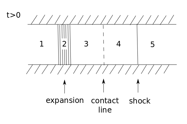
Region 1 & 5 - left and right sides of initial states
Region 2 - expansion or rarefaction wave (x-dependent state)
Regions 3 & 4 - steady states independent of x within the region (uniform)

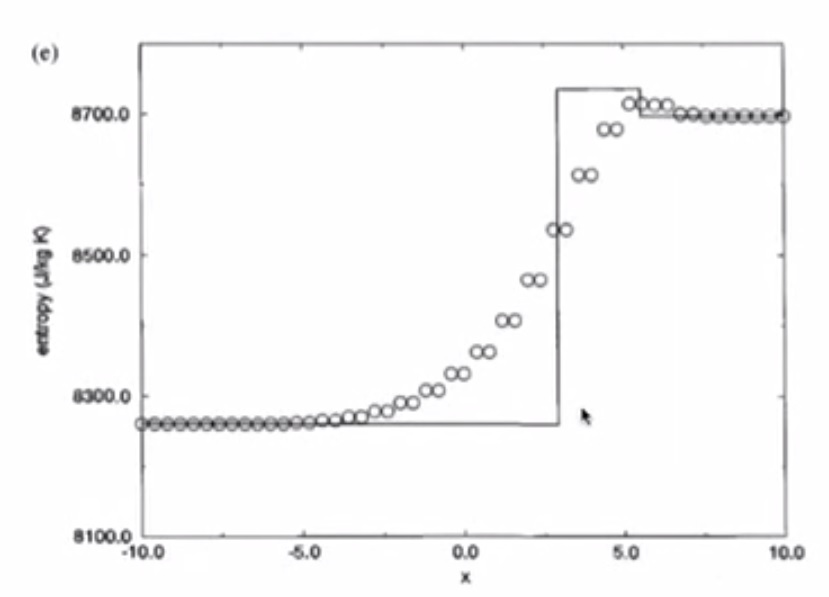
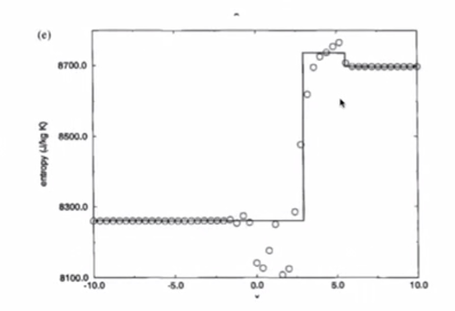
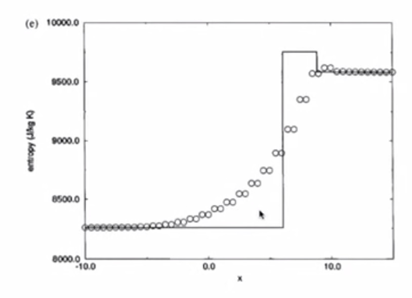
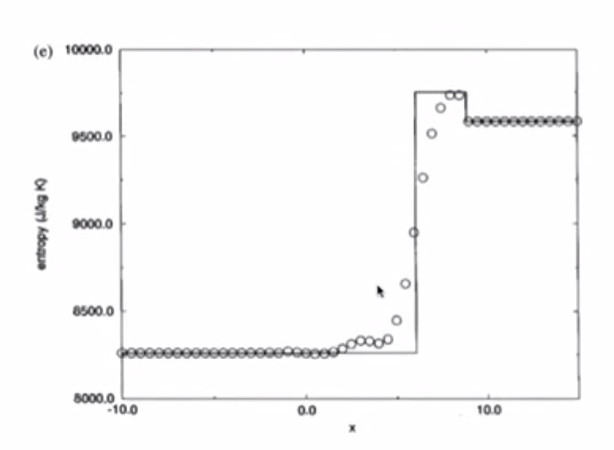
Contact line between 3 and 4 separates fluids of different entropy (but they have the same pressure and velocity) i.e. it’s an invisible line - e.g. two fluids one side with water and the other with dye - contact line is moving.

\[p_3 = p_4\]

\[u_3 = u_4\]

4.4. Sod’s Test Number 1 ¶

Unknowns:

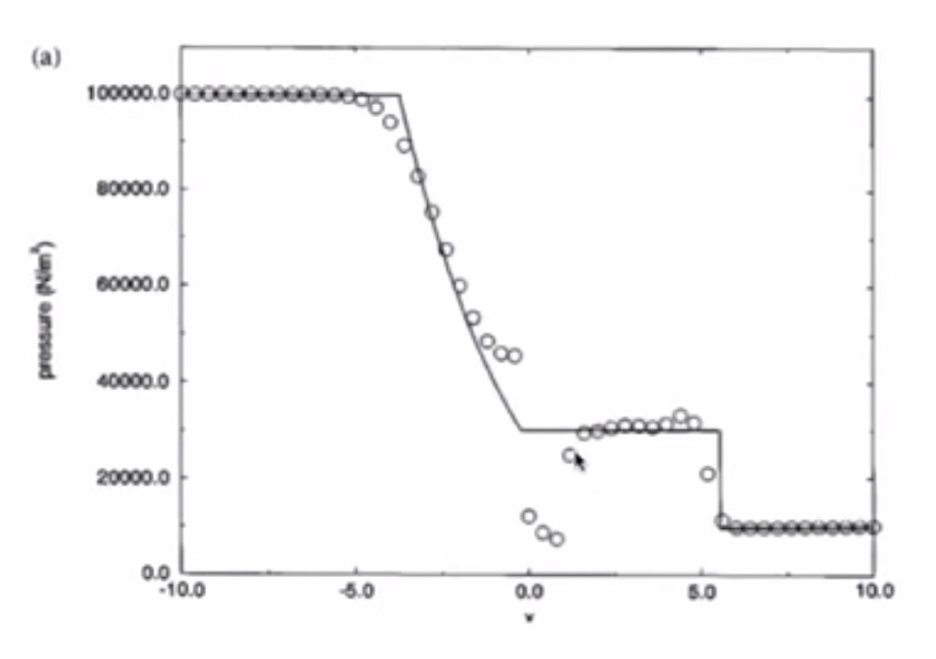
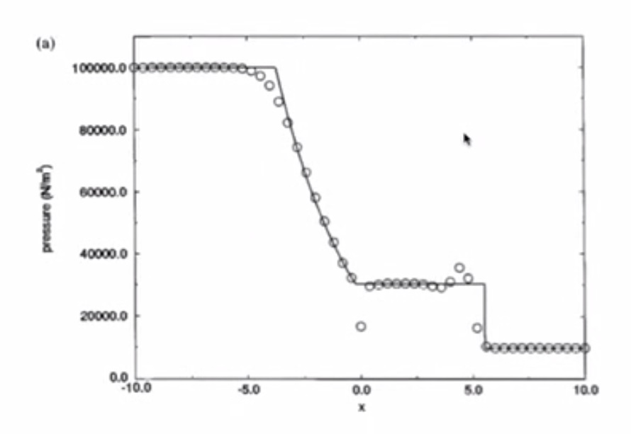
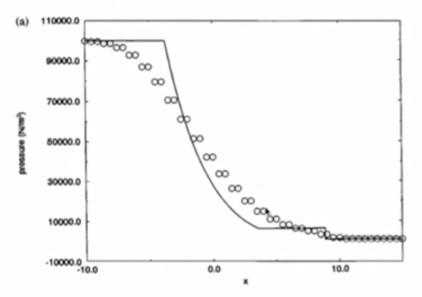
Pressure
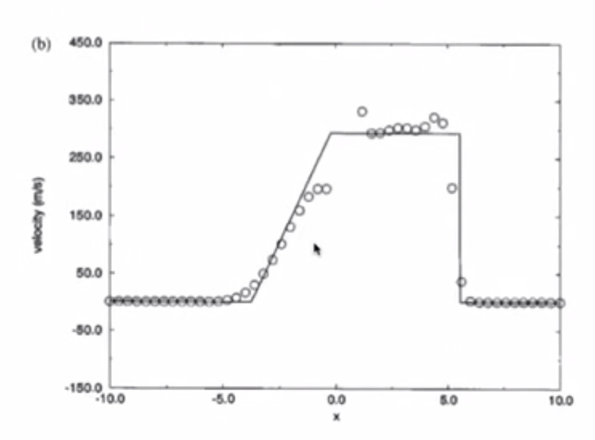
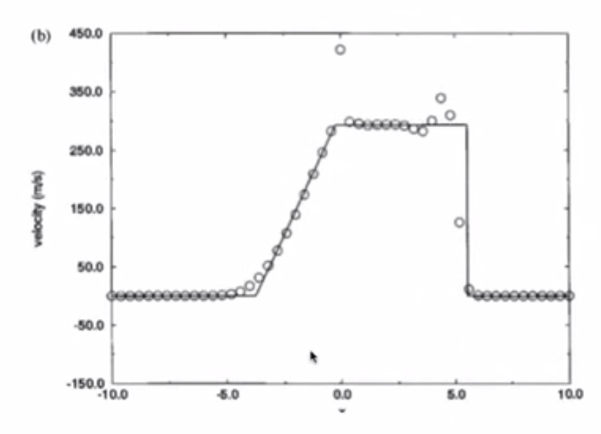
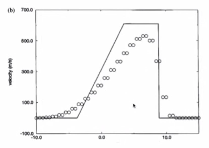
Velocity
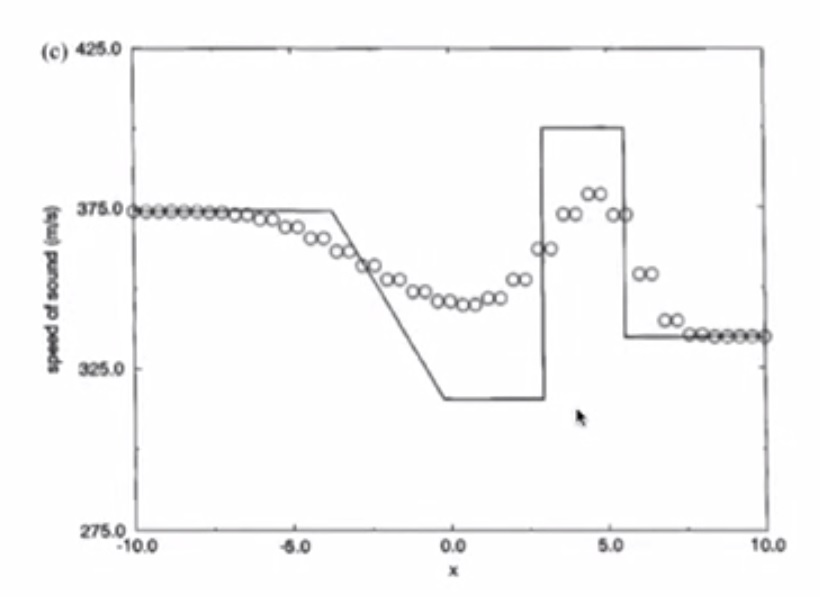
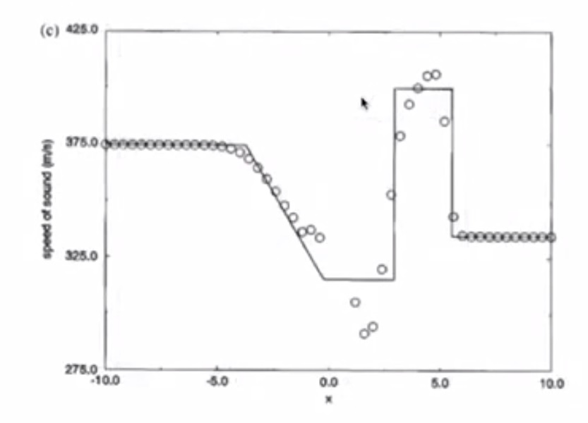
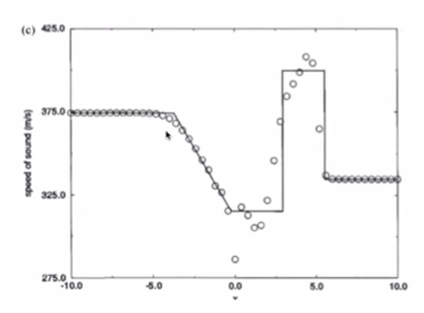
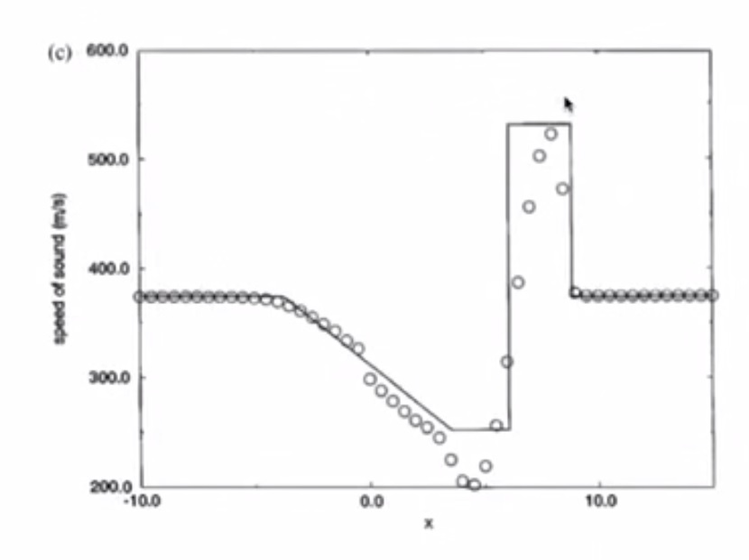
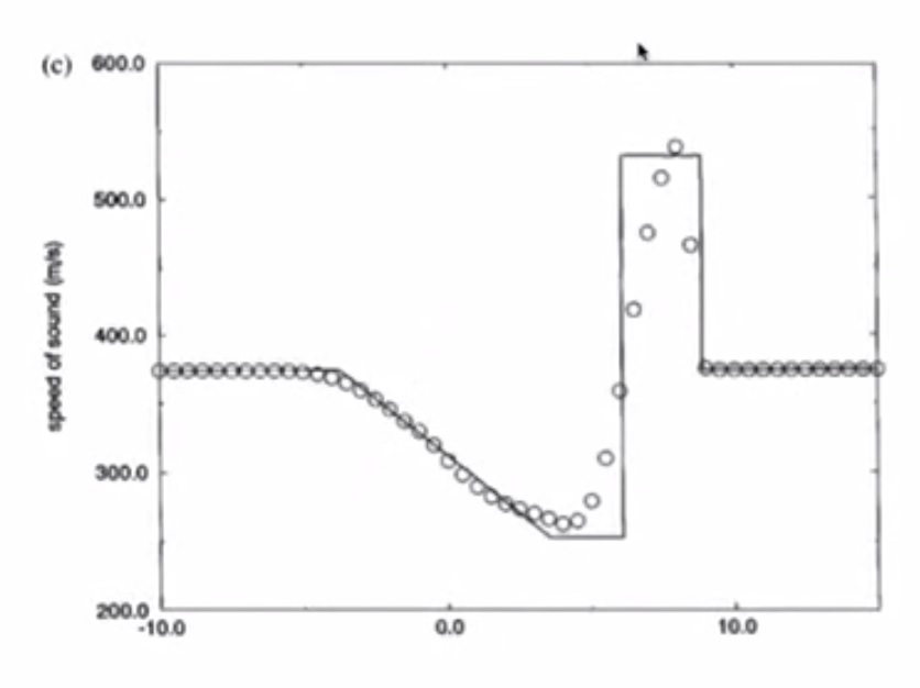
Speed of sound
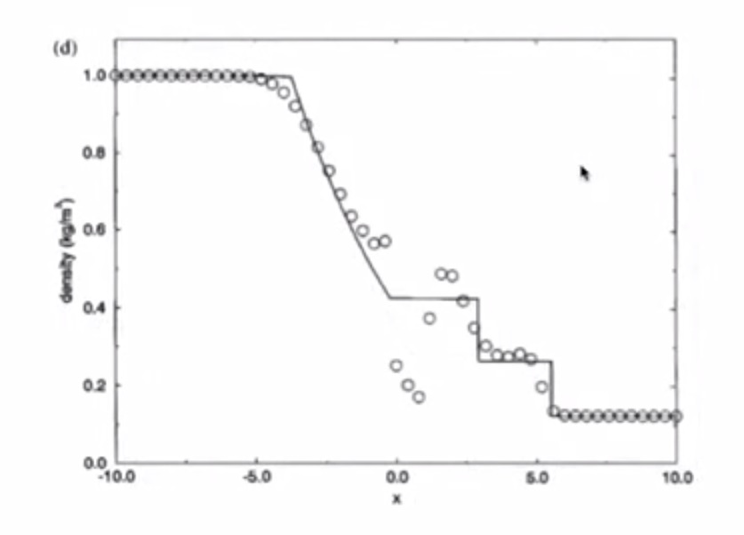
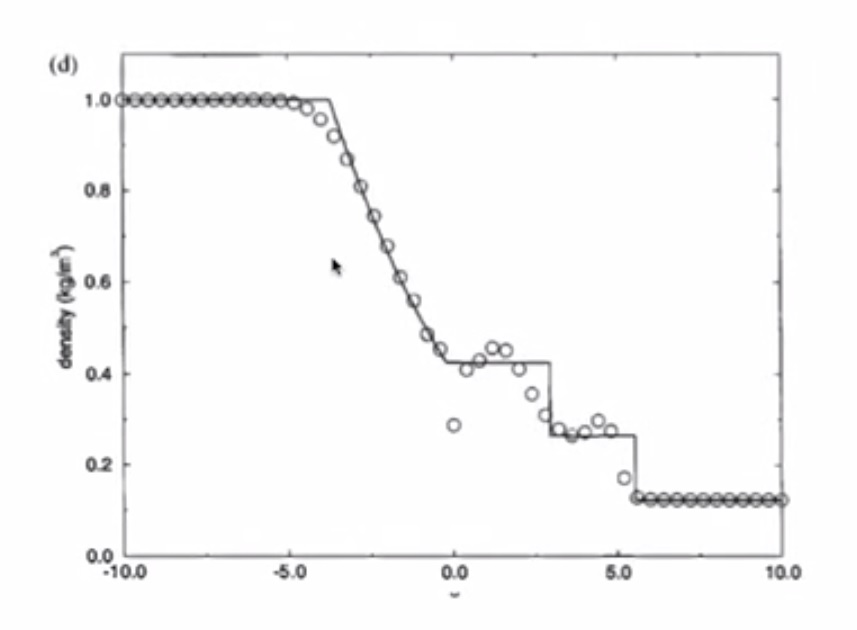
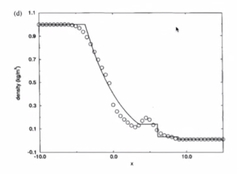
Density
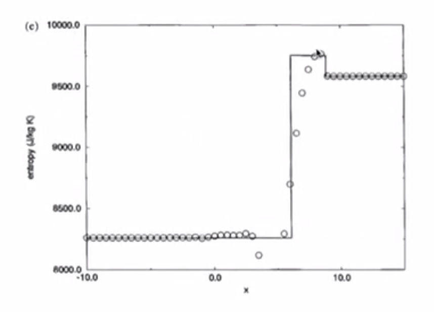
Entropy
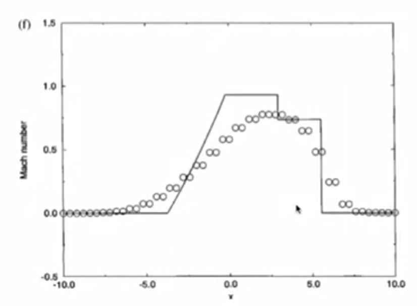
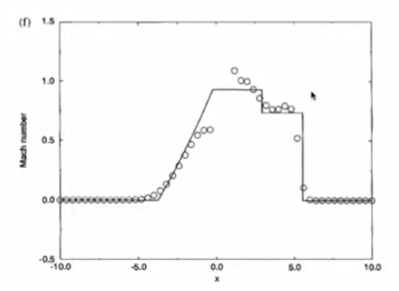
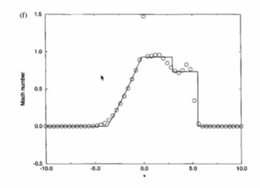
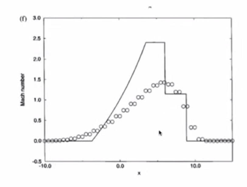
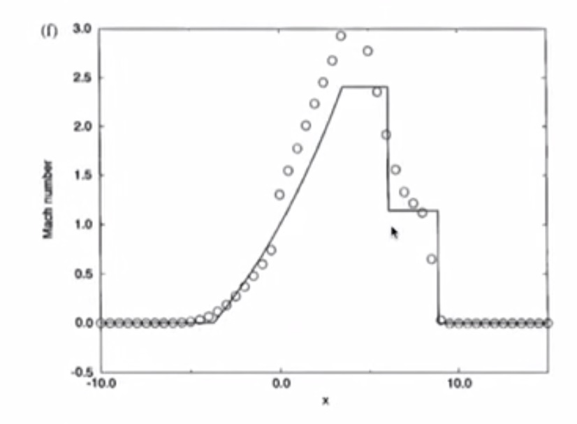
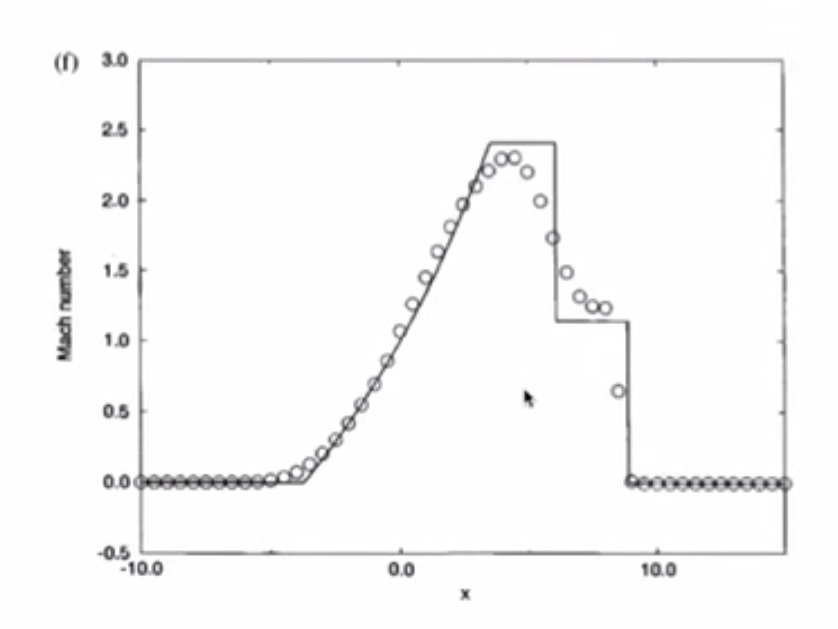
Mach Number

Can also use Euler Equations in Primitive Form with:

Pressure
Velocity
Density

Vector notation for the Euler Equations with Primitive Variables, \(p, u, \rho\)

4.4.1. Initial Conditions ¶

\[\begin{split}\mathbf{V}(x,0) = \begin{cases} \mathbf{V}_L \quad x \lt 0 \\ \mathbf{V}_R \quad x \ge 0 \end{cases}\end{split}\]

\[\begin{split}\mathbf{V}_L = \begin{bmatrix} \rho_L \\ u_L \\ p_L \end{bmatrix} = \begin{bmatrix} 1 kg/m^3 \\ 0 m/s \\ 100 kN/m^2 \end{bmatrix}\end{split}\]

\[\begin{split}\mathbf{V}_R = \begin{bmatrix} \rho_R \\ u_R \\ p_R \end{bmatrix} = \begin{bmatrix} 0.125 kg/m^3 \\ 0 m/s \\ 10 kN/m^2 \end{bmatrix}\end{split}\]

Everything is quiet until you break the diaphragm (u=0)
The pressure ratio is 10

4.4.2. Discretisation ¶

N = 50 points in [-10m, 10m]
\(\Delta x\) = 20m / 50 = 0.4m
Initial CFL = 0.3
Initial wave speed = 374.17m/s
Timestep \(\Delta t\) = 0.4(0.4/374.17) = 4.276 \(\times 10^{-4}\)
\(\Delta t / \Delta x\) = 1.069 \(\times 10^{-3}\)

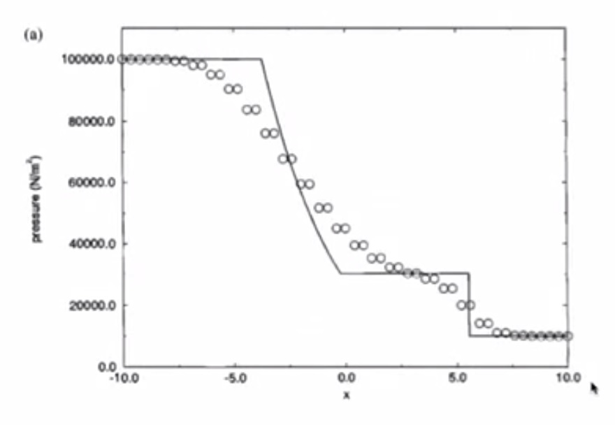
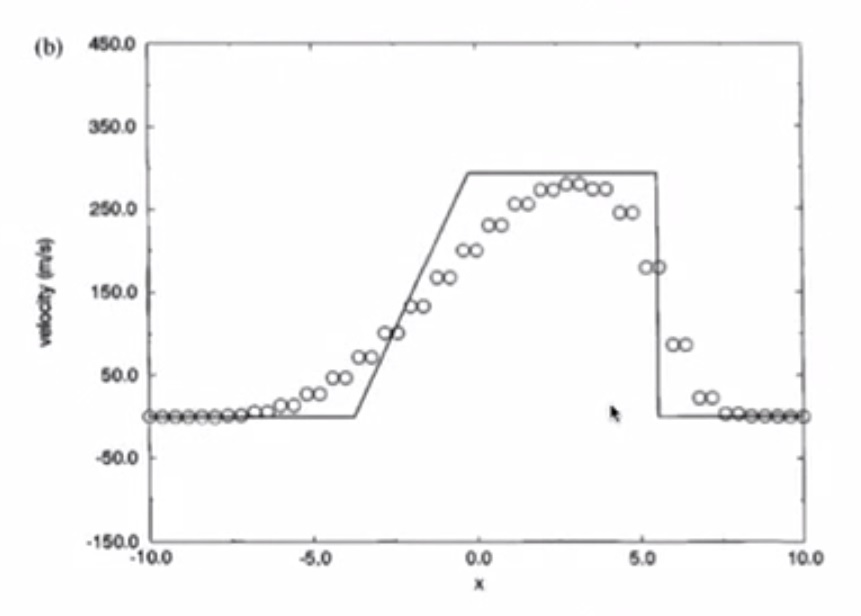
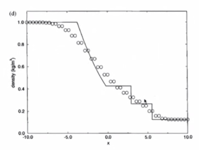
Solution at t = 0.01s (in about 23 timesteps)

Now the problem is described, the numerical schemes can be applied.

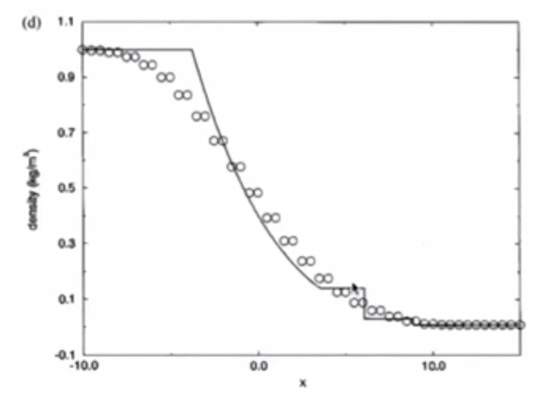
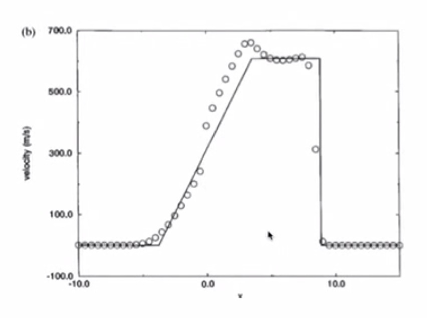
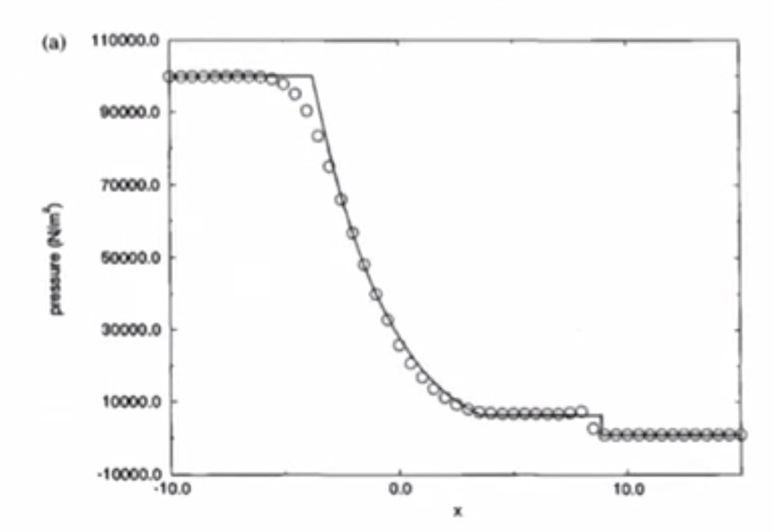
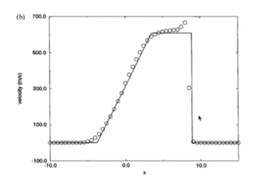
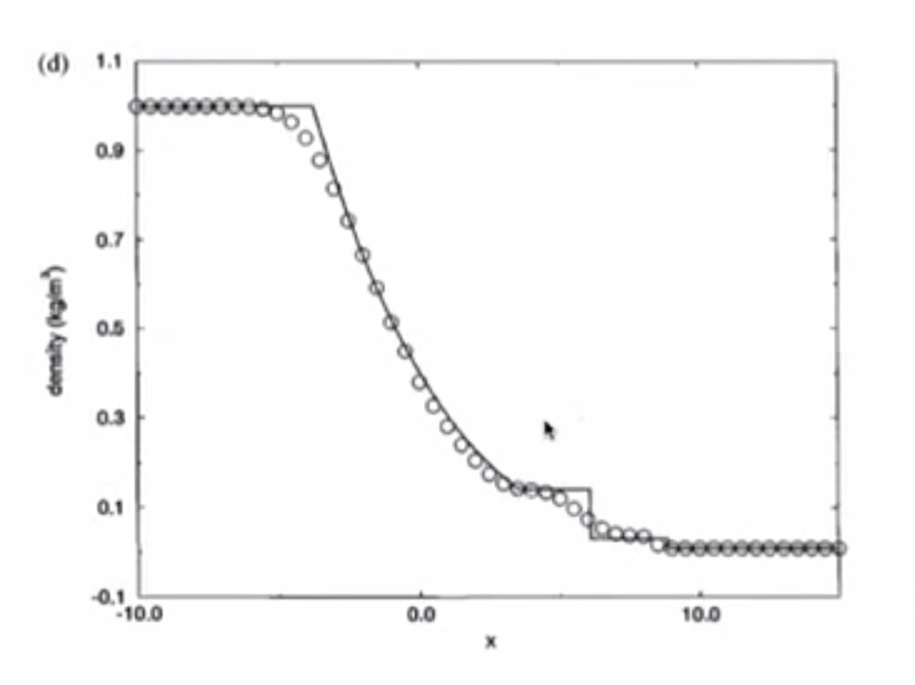
4.5. Sod’s Test Number 2 ¶

Unknowns are same as Test Number 1

4.5.1. Initial Conditions ¶

\[\begin{split}\mathbf{V}_L = \begin{bmatrix} \rho_L \\ u_L \\ p_L \end{bmatrix} = \begin{bmatrix} 1 kg/m^3 \\ 0 m/s \\ 100 kN/m^2 \end{bmatrix}\end{split}\]

\[\begin{split}\mathbf{V}_R = \begin{bmatrix} \rho_R \\ u_R \\ p_R \end{bmatrix} = \begin{bmatrix} 0.01 kg/m^3 \\ 0 m/s \\ 1 kN/m^2 \end{bmatrix}\end{split}\]

Pressure ratio is 100 - this test is harder