2. 1D First-order Non-Linear Convection - The Inviscid Burgers’ Equation
2.1. Understand the Problem
- What is the final velocity profile for 1D non-linear convection when the initial conditions are a square wave and the boundary conditions are constant?
- 1D non-linear convection is described as follows:
\[{\partial u \over \partial t} + u {\partial u \over \partial x} = 0\]
- This equation is capable of generating discontinuities (shocks)
2.2. Formulate the Problem
- Same as Linear Convection
2.3. Design Algorithm to Solve Problem
2.3.1. Space-time discretisation
- Same as Linear Convection
2.3.2. Numerical scheme
- Same as Linear Convection
2.3.3. Discrete equation
\[{{u_i^{n+1} - u_i^n} \over {\Delta t}} + c {{u_i^n - u_{i-1}^n} \over \Delta x}=0\]
2.3.4. Transpose
\[u_i^{n+1} = u_i^n - c{\Delta t \over \Delta x}(u_i^n - u_{i-1}^n)\]
2.3.5. Pseudo-code
- Very similar to Linear Convection
2.4. Implement Algorithm in Python
- Very similar to Linear Convection

2.5. Conclusions
2.5.1. Why isn’t the square wave maintained?
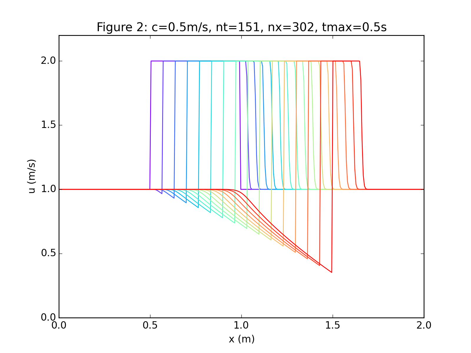
- The first order backward differencing scheme in space still creates false diffusion as before.
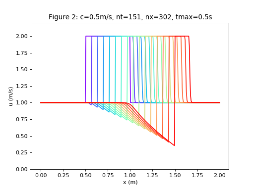
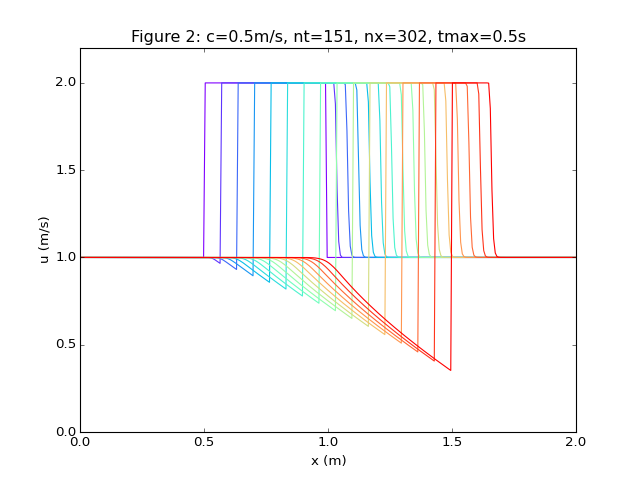
- However, due to the non-linearity in the governing equation, if the spatial step is reduced, the solution can develop shocks, see Figure 2.
- Clearly a square wave is not best represented with the inviscid Burgers Equation.
2.5.2. Why does the wave shift to the right?
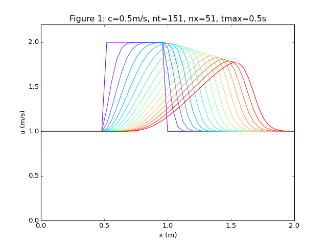
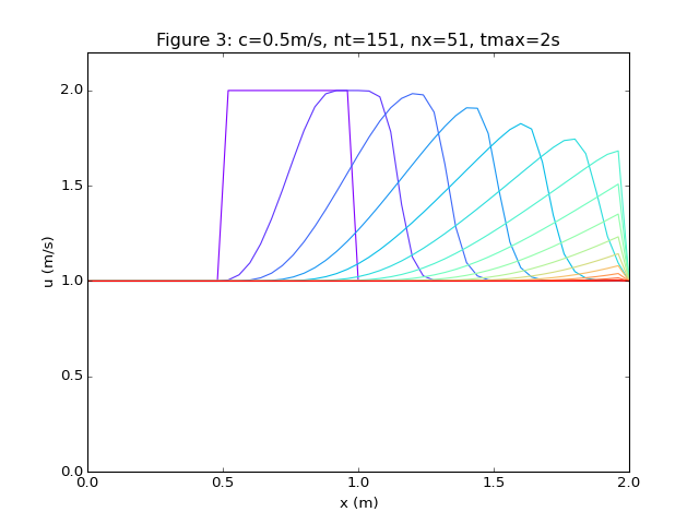
- The square wave is being convected by the velocity, u which is not constant.
- The greatest shift is where the velocity is greatest, see Figure 1
2.5.3. What happens at the wall?
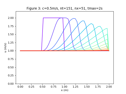
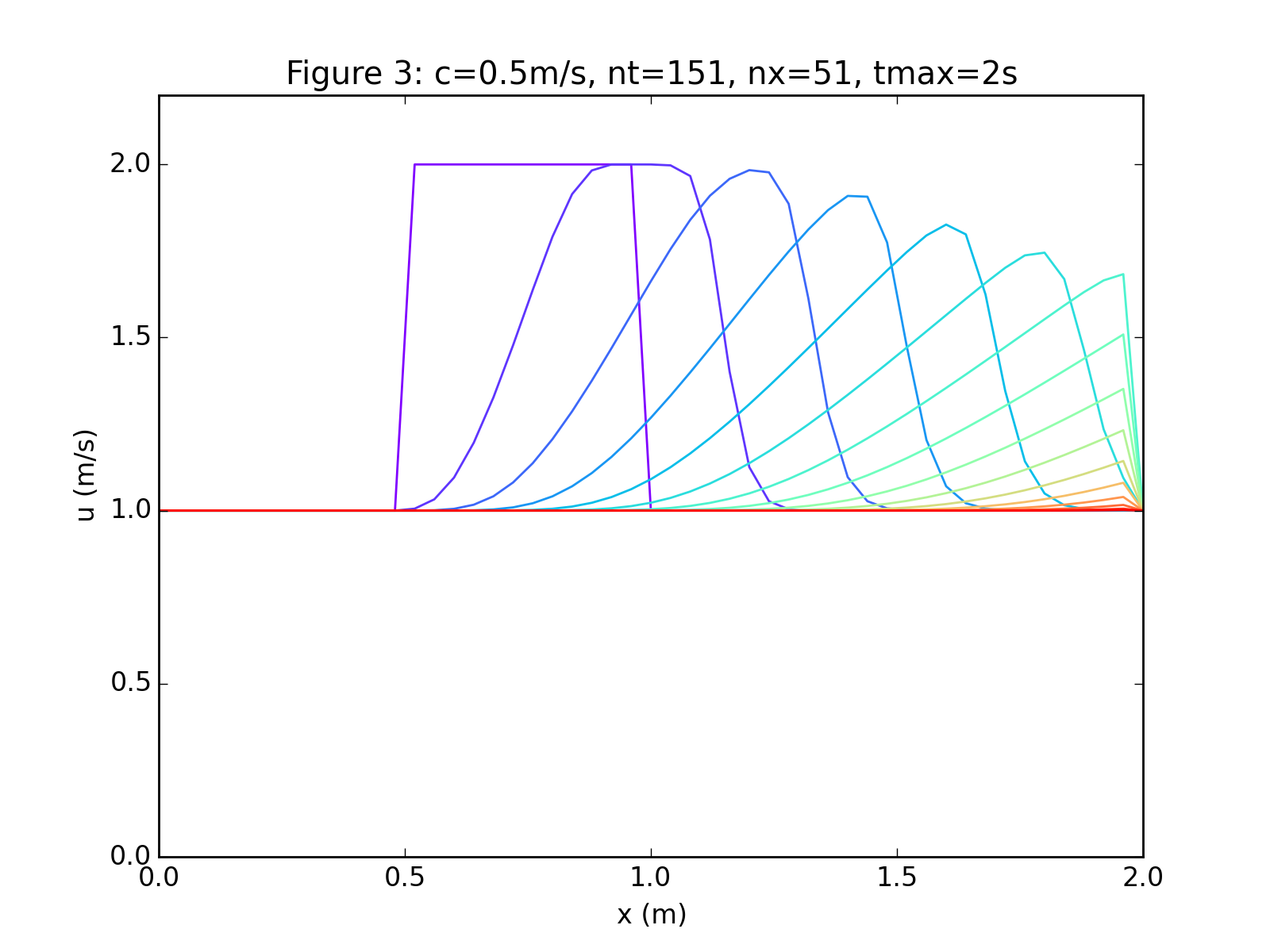
- As there is no viscosity, there is a non-physical change in the profile near the wall, see Figure 3.
- Comparing this with the linear example, there is clearly much more numerical diffusion in the non-linear example, perhaps due to the convective term being larger, causing a greater magnitude in numerical diffusion.